An integrated phylogenomic approach for potential host-parasite associated evolution of monstrilloid copepods
Jeon D., Song C.-u., Jeong H.G., Ohtsuka S., Lee W., Soh H.Y., Eyun S.
Oceanography and Marine Biology: An Annual Review 62:350-375

— Figures and Tables (Colored and High resolution) —
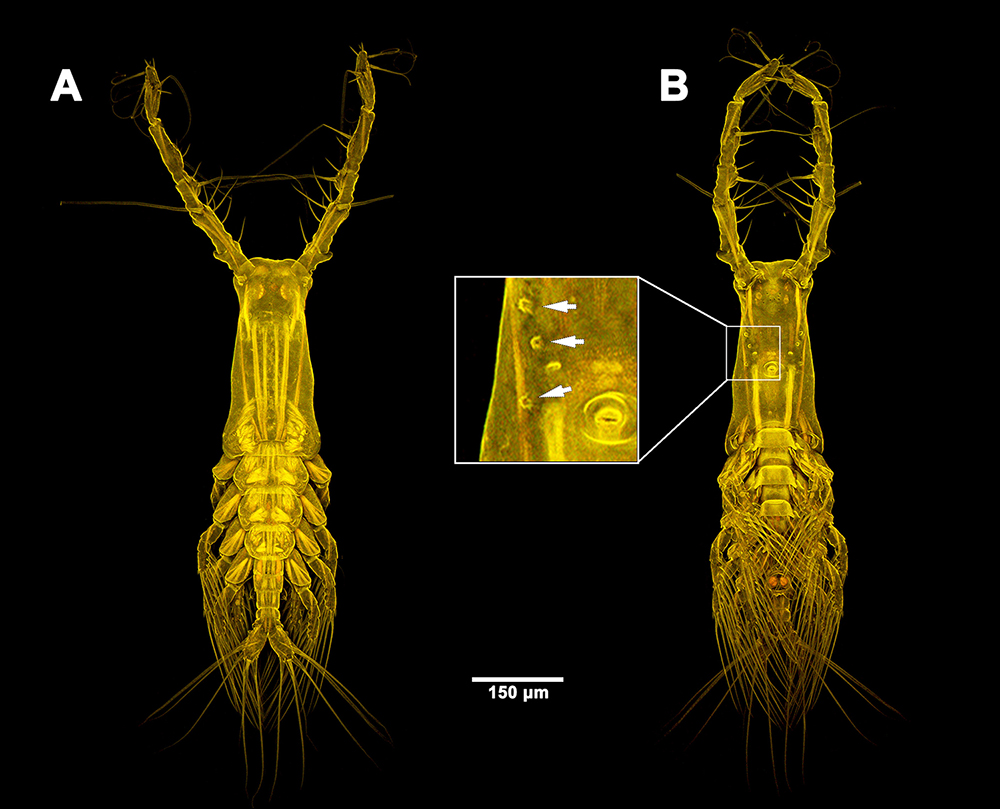
Figure 1. Confocal laser scanning microscope image of adult male Monstrilla grandis. (A) habitus, dorsal view. (B) habitus, ventral view. The inset illustrates three scars (arrows) on the right ventral side of cephalothorax. Monstrilloid specimen preserved in 4% borax buffered formalin was stained by dissolved Congo Red for 24h at room temperature. The stained specimen was washed in distilled water until no solute staining dye was present and then observed on a confocal laser scanning microscope Leica TCS5 (Leica, Germany) equipped with an optical microscope Leica DM5000 (Leica) using three visible lasers (Argon, DPSS, and HeNe). Scale bar in a micrometer. Microphotographs were provided by Dr. Seunghan Lee (Marine Act co., Korea).
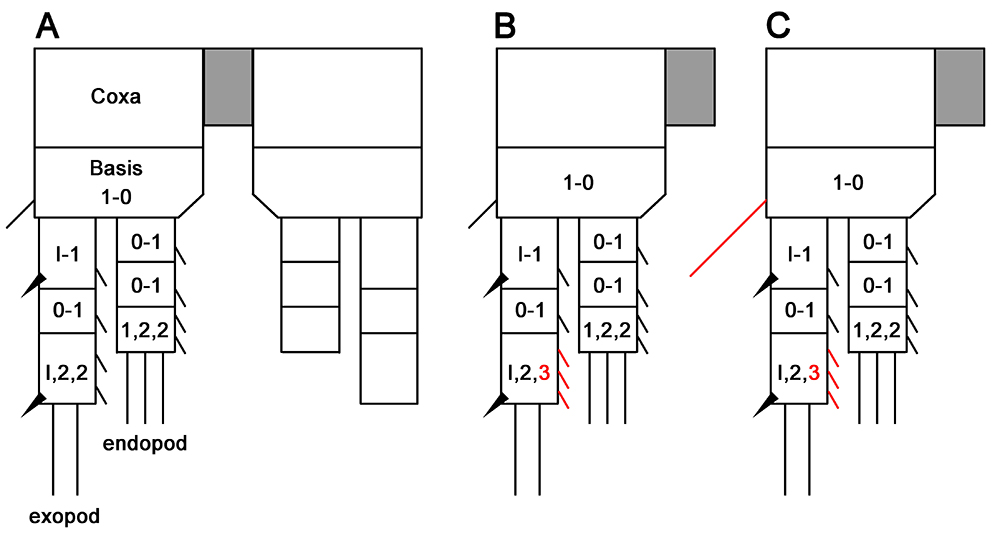
Figure 2. Schematic diagrams of swimming legs 1-4 with setation patterns. (A) pair of leg 1, each conjoined by an intercoxal sclerite (grey box). (B) legs 2 and 4. (C) leg 3. Arrowheads and lines indicate spinous and setal elements, respectively. Red-coloured numbers and elements the difference from the leg 1. Lines for setae, except for the basal setae, do not represent their actual length or its ratio. Nomenclatural terms for describing the setation were adopted from Sewell (1949): Roman and Arabic numerals indicate the number of spines and setae, repectively.
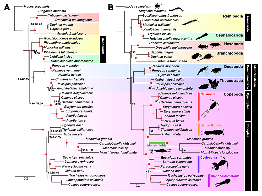
Figure 3. Phylogenies of 21 copepod and 19 other arthropod species inferred from 25 nuclear protein-coding genes. (A) Tree inferred using RAxML-NG and MrBayes. The numbers near the branching points indicate the maximum-likelihood bootstrap support values (BS, in percentage) and Bayesian posterior probabilities (PP, in probability) in order of BS/PP. (B) Tree inferred using IQ-TREE2 with the protein mixture model, C20. The numbers near the branching points indicate BS values. The red dots at the nodes indicate that BS and PP are 100% and 1.00, respectively. Non-pancrustacean species (Ixodes scapularis) is used as the outgroup. The clade names (Xenocarida, Communostraca, and Multicrustacea) are adopted from Regier et al. (2010).
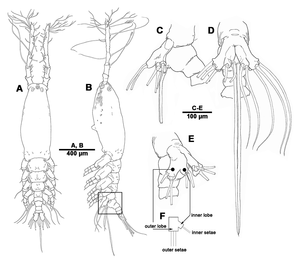
Figure 4. Monstrilla grandis, adult female. (A) habitus, dorsal view. (B) habitus, lateral view. Urosomal part bearing fifth leg highlighted in box. (C) Detail of urosomal part in B, lateral view. (D) Urosome showing a pair of fifth legs, ventral view. (E) First urosomal somite bearing a pair of fifth legs, lateroventral view. Ovigerous spines not presented. (F) Diagrammatic representation of fifth leg (cf. Figure 5).
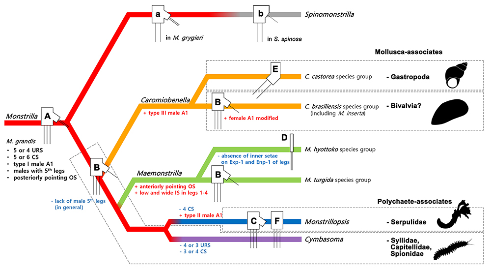
Figure 5. Schematic diagram of morphological divergence of the female fifth leg. The acquisition of new features (in red with '+' marks) and morphological oligomerization (in blue with '-' marks) are shown along the branches. The most plesiomorphic characters from Monstrilla grandis were provided (in black). The host groups utilised by the monstrilloid genera were presented in dashed boxes mapping on the appropriate branches. (A) bilobed leg with 3 outer and 2 inner setae in M. grandis; (B) bilobed leg with 3 outer and 1 inner seta, in the majoritiy of Monstrilla, Maemonstrilla turgida species-group and Caromiobenella brasiliensis species-group; (C) bilobed leg with 3 outer setae, inner lobe unarmed, in the majority of Cymbasoma and Monstrillopsis; (D) a long, rod-shaped leg with 2 apical setae, in the Maemonstrilla hyottoko species-group; (E) unilobed leg bent outward at half, in Caromiobenella species; (F) unilobed leg with 3 setae, inner lobe almost rudimentary or absent, in some Cymbasoma (e.g., C. bowmani) (Suárez-Morales & Gasca 1998) and Monstrillopsis (e.g., M. planifrons) (Delaforge et al. 2017); (a) bilobed leg with 2 outer and 2 inner setae in Monstrilla grygieri (Suárez-Morales 2000); (b) unilobed leg with 2 apical and 1 inner seta in Spinomonstrilla spinosa (Park 1967, Suárez-Morales 2019). Females of Australomonstrillopsis have not been reported. Branch colour of red, orange, green, blue, purple, and grey indicate the lineage of the genus Monstrilla, Caromiobenella, Maemonstrilla, Monstrillopsis, Cymbasoma, and Spinomonstrilla, respectively. Abbreviations used: URS, urosomal somites; CS, caudal setae; A1, antennules; OS, ovigerous spines; IS, intercoxal sclerites; Exp-1, first exopodal segment of leg; Enp-1, first endopodal segment of leg.
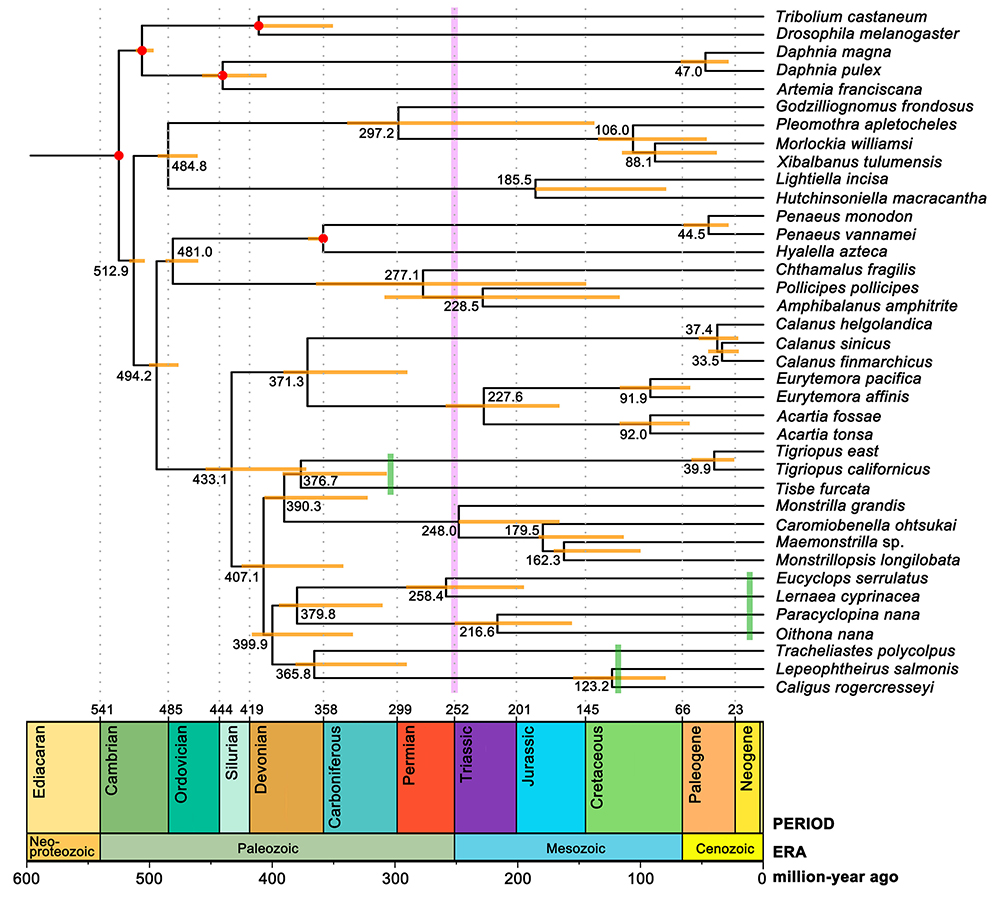
Figure 6. Estimated divergence times for arthropod species inferred using LSD2 (ver. 1.10) (To et al. 2016) with five non-copepod calibration points indicated by red dots. Orange horizontal bars near nodes indicate 95% confidence intervals and green vertical bars indicate the fossil records of Copepoda. Purple vertical bar indicates the Permian-Triassic extinction. The geological time scale is prepared according to the International Chronostratigraphic Chart (http://www.stratigraphy.org).
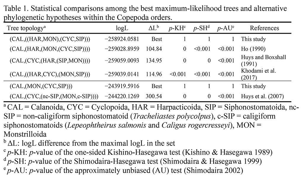
Table 1. Statistical comparisons among the best maximum-likelihood trees and alternative phylogenetic hypotheses within the Copepoda orders.
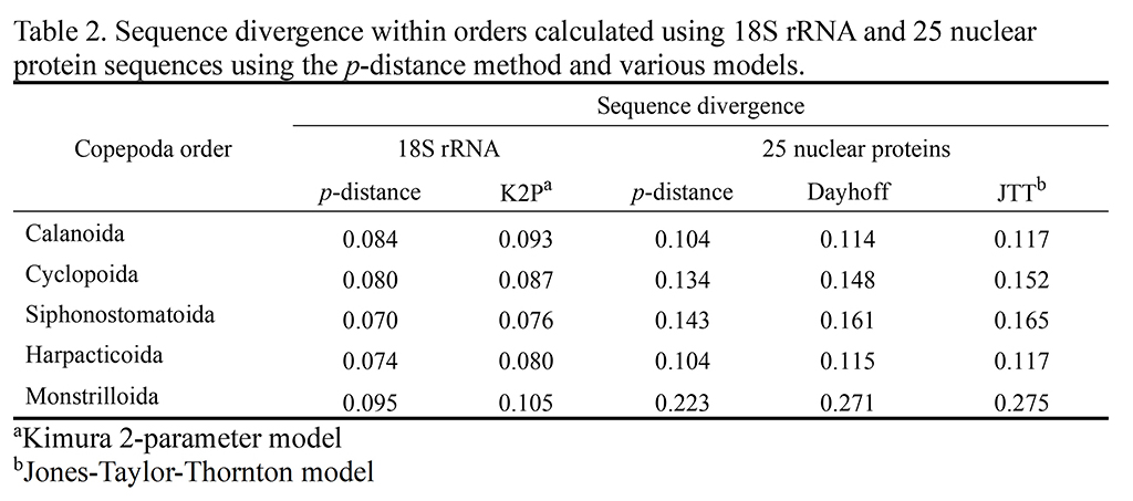
Table 2. Sequence divergence within orders calculated using 18S rRNA and 25 nuclear protein sequences using the p-distance method and various models.
— Supplemental Figures and Tables (Colored and High resolution) —
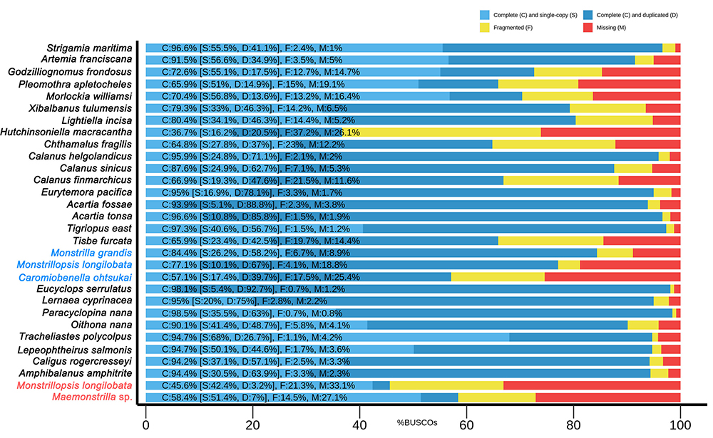
Figure S1. Results of BUSCO assessment for 28 transcriptomes and 2 genomes from 29 arthropod species. Each x- and y-axis shows the percentage of BUSCO genes in each assembly and the list of arthropod species, respectively. The names of the monstrilloid species in blue indicate the transcriptome assemblies and those in red indicate genome assemblies. The reference database for BUSCO (ver. 5.3.2) was the Arthropoda lineage dataset (arthropoda_odb10, as of September 2020) containing a total 1,013 marker genes.
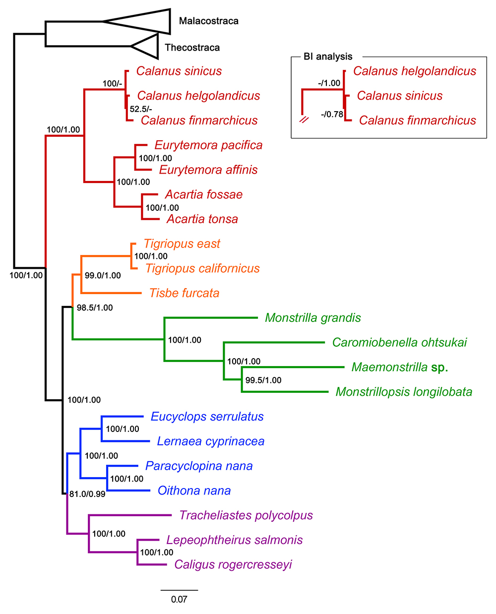
Figure S2. Phylogenetic tree based on 25 protein sequences from five copepod orders with the communostracan taxa as outgroups. Nodal support values of BS (in percentage)/PP (in probability) are presented near branching points. Note that ML and BI analyses showed different subtrees for the genus Calanus; therefore, PP values are separately presented in the inset (BI analysis). Colour indexes for copepod orders: Calanoida (red), Harpacticoida (orange), Monstrilloida (green), Cyclopoida (blue), and Siphonostomatoida (purple).
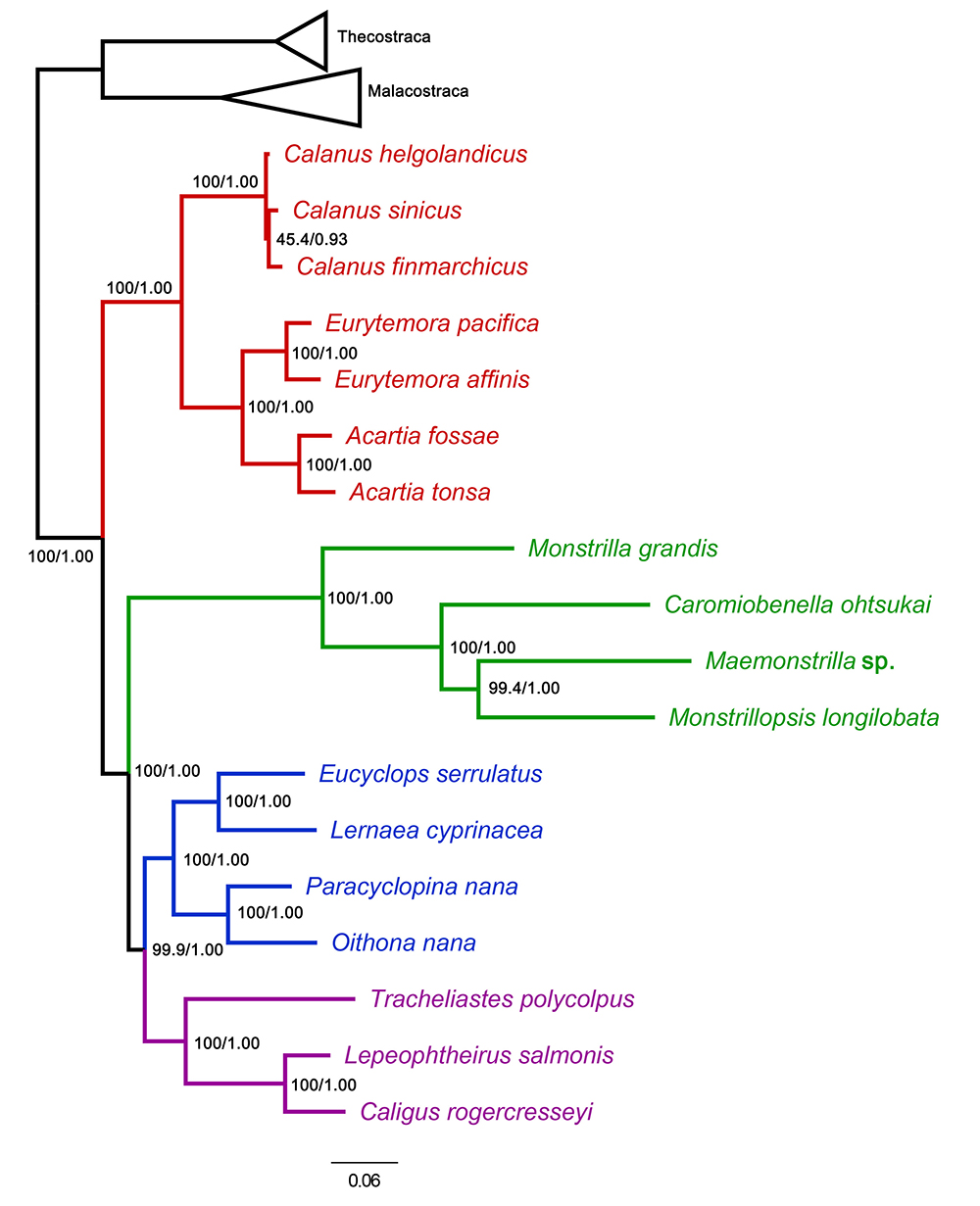
Figure S3. Phylogenetic tree based on 25 protein sequences from four copepod orders with the communostracan taxa as outgroups. Nodal support values of BS (in percentage)/PP (in probability) are presented near branching points. Colour indexes for copepod orders: Calanoida (red), Monstrilloida (green), Cyclopoida (blue), and Siphonostomatoida (purple).
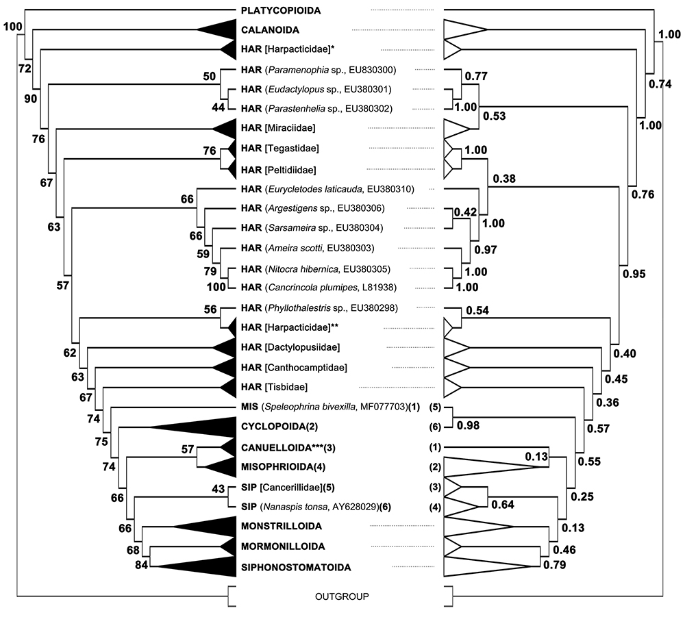
Figure S4. Phylogenetic cladograms of Copepoda reconstructed based on 18S rRNA sequences with two communostracan taxa, Squilla empusa (Malacostraca) and Berndtia purpurea (Thecostraca) as outgroups. ML (on the left) and BI (on the right) trees are presented with the support values of the BS (in percentage) and PP (in probability) near the branching points, respectively. Some taxon groups were collapsed at the order- or family-levels. Family names are in square brackets and species names and GenBank accession numbers are in parentheses. HAR = Harpacticoida; MIS = Misophrioida; SIP = Siphonostomatoida. *: Harpacticidae consisting of Tigriopus species, **: Harpacticidae consisting of Harpacticus and Zaus species, and ***: the name was adopted from Khodami et al. (2017).
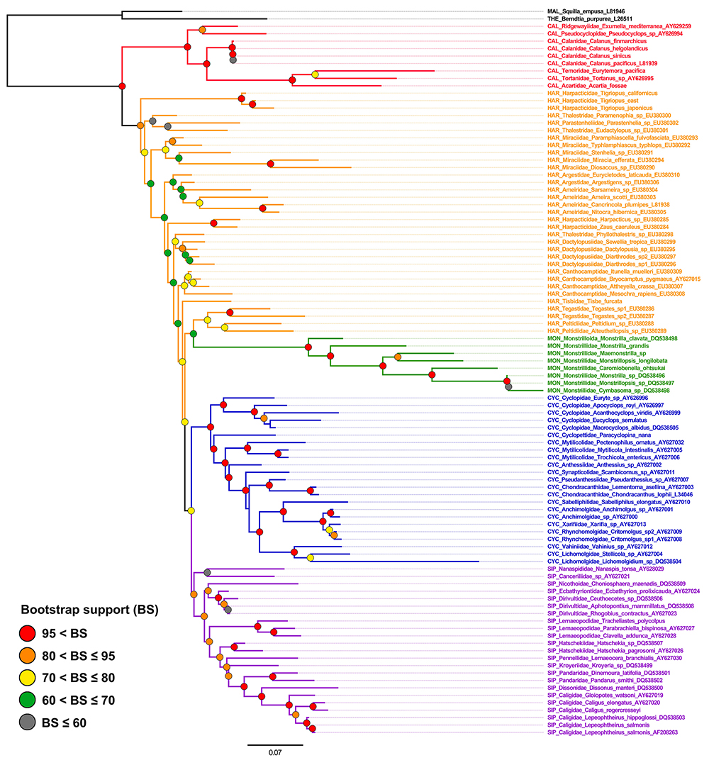
Figure S5. Maximum-likelihood phylogenetic tree reconstructed based on 18S rRNA sequences of five copepod orders with two communostracan taxa, Squilla empusa (Malacostraca) and Berndtia purpurea (Thecostraca) as outgroups. Bootstrap supporting values are presented with dots in different colour indexes. Colour indexes for copepod orders: Calanoida (red), Harpacticoida (orange), Monstrilloida (green), Cyclopoida (blue), and Siphonostomatoida (purple).
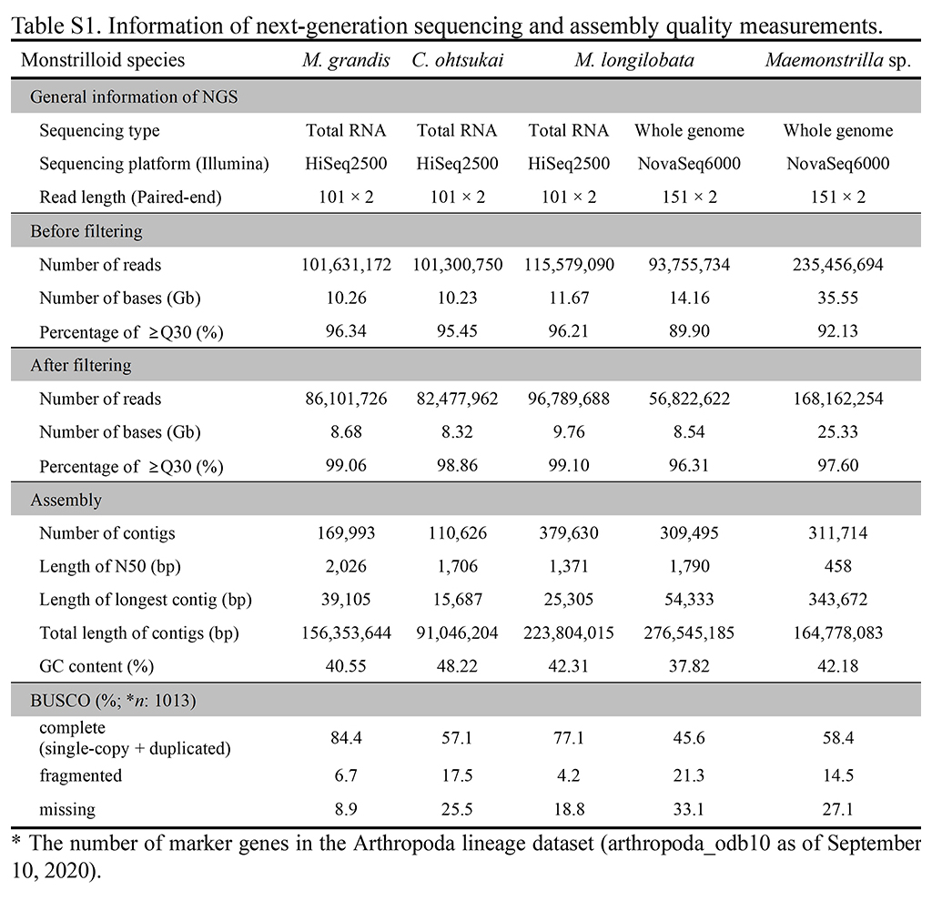
Table S1. Information of next-generation sequencing and assembly quality measurements.
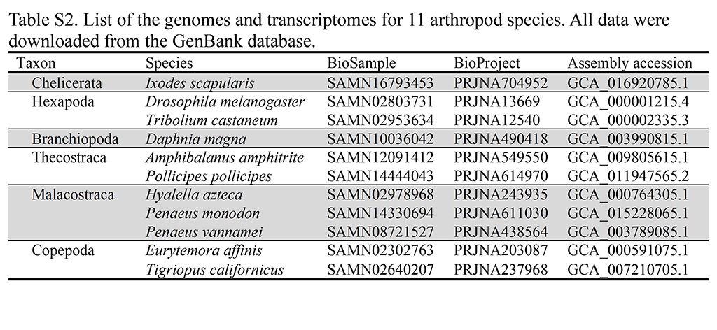
Table S2. List of the genomes and transcriptomes for 11 arthropod species. All data were downloaded from the GenBank database.
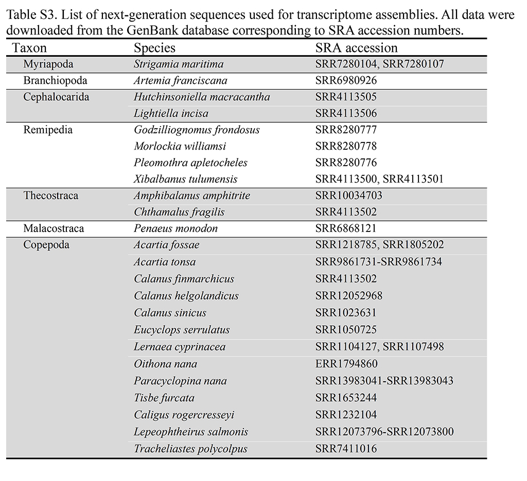
Table S3. List of next-generation sequences used for transcriptome assemblies. All data were downloaded from the GenBank database corresponding to SRA accession numbers.
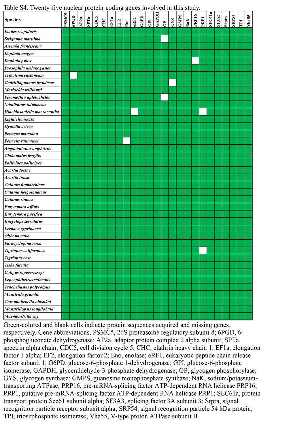
Table S4. Twenty-five nuclear protein-coding genes involved in this study.
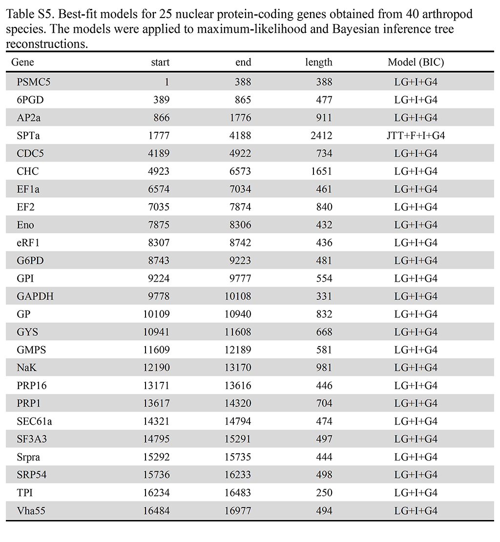
Table S5. Best-fit models for 25 nuclear protein-coding genes obtained from 40 arthropod species. The models were applied to maximum-likelihood and Bayesian inference tree reconstructions.
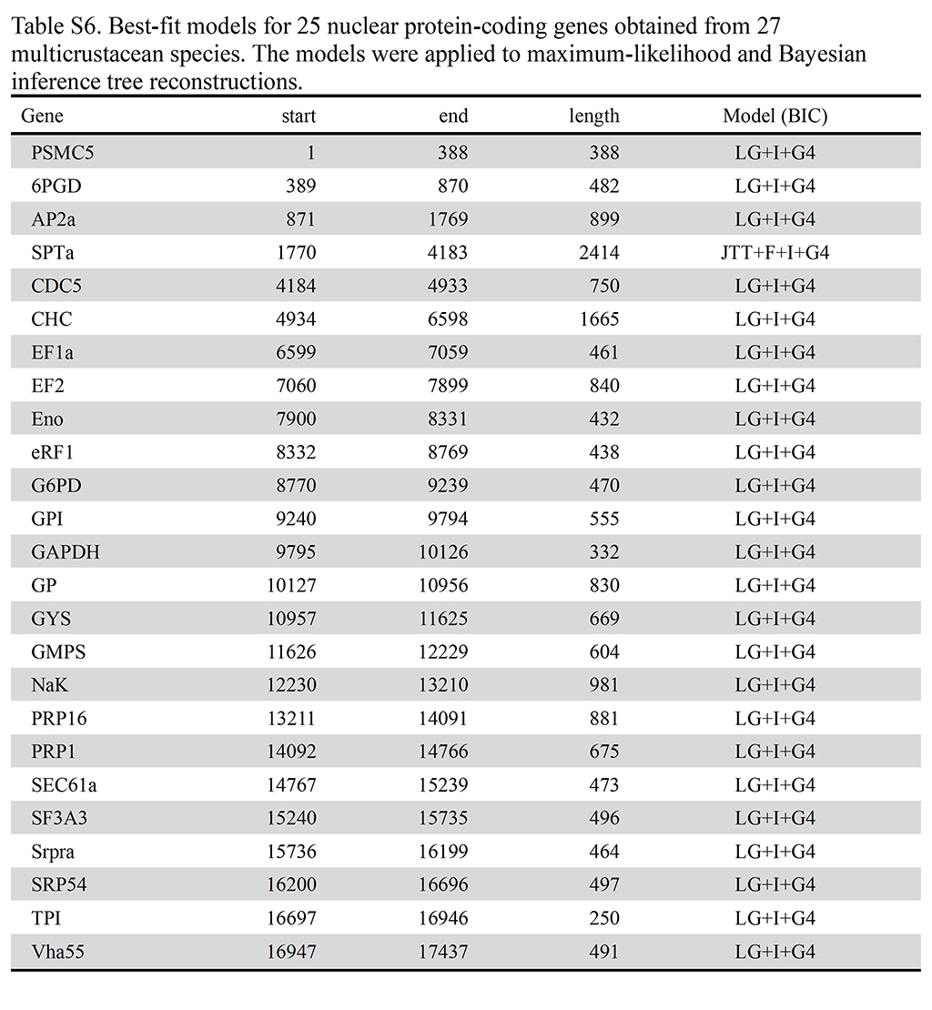
Table S6. Best-fit models for 25 nuclear protein-coding genes obtained from 27 multicrustacean species. The models were applied to maximum-likelihood and Bayesian inference tree reconstructions.
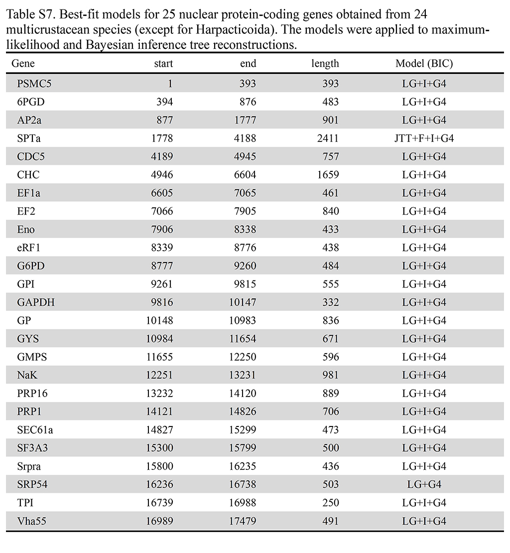
Table S7. Best-fit models for 25 nuclear protein-coding genes obtained from 24 multicrustacean species (except for Harpacticoida). The models were applied to maximum-likelihood and Bayesian inference tree reconstructions.
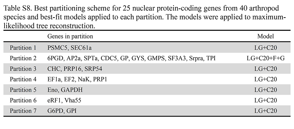
Table S8. Best partitioning scheme for 25 nuclear protein-coding genes from 40 arthropod species and best-fit models applied to each partition. The models were applied to maximum-likelihood tree reconstruction.
— Copepod sequences used —
- Additional File 1. All 25 nuclear protein-coding gene sequences used for phylogenetic analyses. (zip)
- Additional File 2. Concatenated protein sequences for phylogenetic tree reconstruction. (zip)
- Protein sequence alignments generated by MAFFT (in fasta format)
- 26S proteasome regulatory subunit 8
- 6-phosphogluconate dehydrogenase
- adaptor protein complex 2 alpha subunit
- spectrin alpha chain
- cell division cycle 5
- clathrin heavy chain 1
- elongation factor 1 alpha
- elongation factor 2
- enolase
- eukaryotic peptide chain release factor subunit 1
- glucose-6-phosphate 1-dehydrogenase
- glucose-6-phosphate isomerase
- glyceraldehyde-3-phosphate dehydrogenase
- glycogen phosphorylase
- glycogen synthase
- guanosine monophosphate synthase
- sodium/potassium-transporting ATPase
- pre-mRNA-splicing factor ATP-dependent RNA helicase PRP16
- putative pre-mRNA-splicing factor ATP-dependent RNA helicase PRP1
- protein transport protein Sec61 subunit alpha
- splicing factor 3A subunit 3
- signal recognition particle receptor subunit alpha
- signal recognition particle 54 kDa protein
- triosephosphate isomerase
- V-type proton ATPase subunit B